10 Modelos de Datos Panel
10.1 Motivación
Denotemos con \(Y_{it}\) el componente o individuo \(i\), \(i = 1, 2, \ldots, N\) en el tiempo \(t\), \(t = 1, 2, \ldots, T\). Típicamente las series de tiempo en forma de panel se caracterizan por ser de dimensión de individuos corta y de dimensión temporar larga.
En general, escribiremos: \[\begin{equation} Y_{it} = \alpha_i + \beta_i X_{it} + U_{it} \end{equation}\]
Donde \(\alpha_i\) es un efecto fijo especificado como: \[\begin{equation} \alpha_i = \beta_0 + \gamma_i Z_i \end{equation}\]
10.2 Pruebas de Raíces Unitarias en Panel
Las pruebas de raíces unitarias para panel suelen ser usadas principalmente en casos macroeconómicos. De forma similar al caso de series univariadas, asumiremos una forma de AR(1) para una serie en panel: \[\begin{equation} \Delta Y_{it} = \mu_i + \rho_i Y_{i t-1} + \sum_{i = 1}^{k_i} \varphi_{ij} \Delta Y_{i t-j} + \varepsilon_{it} (\#eq:eq_AR_Panel) \end{equation}\]
Donde \(i = 1, \ldots, N\), \(t = 1, \ldots, T\) y \(\varepsilon_{it}\) es una v.a. iid que cumple con: \[\begin{eqnarray*} \mathbb{E}[\varepsilon_{it}] & = & 0 \\ \mathbb{E}[\varepsilon_{it}^2] & = & \sigma^2_i < \infty \\ \mathbb{E}[\varepsilon_{it}^4] & < & \infty \end{eqnarray*}\]
Al igual que en el caso univariado, en este tipo de pruebas buscamos identificar cuando las series son I(1) y cuando I(0). Pasra tal efecto, la prueba de raíz unitaria que utilizaremos está basada en una prueba Dickey-Fuller Aumentada en la cual la hipótesis nula (\(H_0\)) es que todas las series en el panel son no estacionarias, es decir, son I(1). Es decir, \[\begin{equation} H_0 : \rho_i = 0 \end{equation}\]
Por su parte, en el caso de la hipótesis nula tenndremos dos:10.3 Ejemplo: Pruebas de Raíces Unitarias en Panel
Dependencies and Setup
Download data from library PLM
data("EmplUK", package="plm")

data("Produc", package="plm")

data("Grunfeld", package="plm")

data("Wages", package="plm")
Describe data: Grunfeld data (Grunfeld 1958) comprising 20 annual observations on the three variables real gross investment (invest), real value of the firm (value), and real value of the capital stock (capital) for 10 large US firms for the years 1935–1954
names(Grunfeld)## [1] "firm" "year" "inv" "value" "capital"
head(Grunfeld)## firm year inv value capital
## 1 1 1935 317.6 3078.5 2.8
## 2 1 1936 391.8 4661.7 52.6
## 3 1 1937 410.6 5387.1 156.9
## 4 1 1938 257.7 2792.2 209.2
## 5 1 1939 330.8 4313.2 203.4
## 6 1 1940 461.2 4643.9 207.2
Invest <- data.frame(split( Grunfeld$inv, Grunfeld$firm )) # individuals in columns

names(Invest)
## [1] "X1" "X2" "X3" "X4" "X5" "X6" "X7" "X8" "X9" "X10"
names(Invest) <- c( "Firm_1", "Firm_2", "Firm_3", "Firm_4",
                    "Firm_5", "Firm_6", "Firm_7", "Firm_8",
                    "Firm_9", "Firm_10" )

names(Invest)
## [1] "Firm_1" "Firm_2" "Firm_3" "Firm_4" "Firm_5" "Firm_6" "Firm_7"
## [8] "Firm_8" "Firm_9" "Firm_10"Plot:
plot(Invest$Firm_1, type = "l", col = 1, ylim = c(0, 1500), lty = 1,
     xlab = "Tiempo", ylab = "Real gross investment")
lines(Invest$Firm_2, type = "l", col = 2, lty = 2)
lines(Invest$Firm_3, type = "l", col = 3, lty = 1)
lines(Invest$Firm_4, type = "l", col = 4, lty = 2)
lines(Invest$Firm_5, type = "l", col = 5, lty = 1)
lines(Invest$Firm_6, type = "l", col = 6, lty = 2)
lines(Invest$Firm_7, type = "l", col = 7, lty = 1)
lines(Invest$Firm_8, type = "l", col = 8, lty = 2)
lines(Invest$Firm_9, type = "l", col = 9, lty = 1)
lines(Invest$Firm_10, type = "l", col = 10, lty = 2)
legend("topleft", legend=c("Firm_1", "Firm_2", "Firm_3", "Firm_4", "Firm_5",
                           "Firm_6", "Firm_7", "Firm_8", "Firm_9", "Firm_10"),
       col = c(1, 2, 3, 4, 5, 6, 7, 8, 9, 10), lty = 1:2)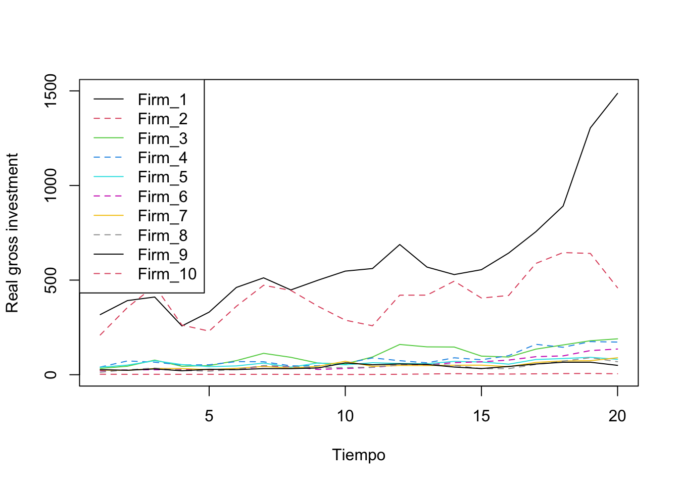
Figure 10.1: Evolución de la inversión por empresa
Unit Root Test: Test specifies the type of test to be performed among Levin et al. (2002), Im et al. (2003), Maddala and Wu (1999) and Hadri (2000)
Consider Levin et al. (2002)
purtest(log(Invest), test = "levinlin", exo = "intercept",
        lags = "AIC", pmax = 4)
## Warning in selectT(l, theTs): the time series is short##
## Levin-Lin-Chu Unit-Root Test (ex. var.: Individual Intercepts)
##
## data: log(Invest)
## z = -0.63214, p-value = 0.2636
## alternative hypothesis: stationaritySame via:
ts_LInvest <- ts(log(Invest), start = 1935, end = 1954, freq = 1)

ts_DLInvest <- diff(ts(log(Invest), start = 1935, end = 1954, freq = 1),
                     lag = 1, differences = 1)
purtest(ts_LInvest, test = "levinlin", exo = "intercept",
        lags = "AIC", pmax = 4)
## Warning in selectT(l, theTs): the time series is short##
## Levin-Lin-Chu Unit-Root Test (ex. var.: Individual Intercepts)
##
## data: ts_LInvest
## z = -0.63214, p-value = 0.2636
## alternative hypothesis: stationarity
summary(purtest(ts_LInvest, test = "levinlin", exo = "intercept",
        lags = "AIC", pmax = 4))
## Warning in selectT(l, theTs): the time series is short## Levin-Lin-Chu Unit-Root Test
## Exogenous variables: Individual Intercepts
## Automatic selection of lags using AIC: 0 - 3 lags (max: 4)
## statistic: -0.632
## p-value: 0.264
##
## lags obs rho trho p.trho sigma2ST sigma2LT
## Firm_1 0 19 0.006034802 0.05068864 0.96193110 0.03592530 0.014769876
## Firm_2 1 18 -0.597193025 -2.95851997 0.03895745 0.05020448 0.014565004
## Firm_3 3 16 -0.257291999 -1.97135237 0.29979349 0.03073205 0.019141095
## Firm_4 0 19 -0.172070863 -1.21388533 0.67084314 0.06196079 0.018454390
## Firm_5 1 18 -0.444726602 -1.69693864 0.43286539 0.04165516 0.006949122
## Firm_6 2 17 0.062922587 0.72626225 0.99275186 0.02442139 0.009212851
## Firm_7 2 17 -0.013830411 -0.08442715 0.94937802 0.03230724 0.007274365
## Firm_8 1 18 -0.365024064 -2.26588313 0.18328720 0.06270208 0.026960667
## Firm_9 0 19 -0.247940802 -1.72877417 0.41668489 0.05073398 0.013291332
## Firm_10 1 18 -0.197003144 -1.52323519 0.52199891 0.07672404 0.062496477
purtest(ts_DLInvest, test = "levinlin", exo = "intercept",
        lags = "AIC", pmax = 4)
## Warning in selectT(l, theTs): the time series is short##
## Levin-Lin-Chu Unit-Root Test (ex. var.: Individual Intercepts)
##
## data: ts_DLInvest
## z = -8.5076, p-value < 0.00000000000000022
## alternative hypothesis: stationarity
summary(purtest(ts_DLInvest, test = "levinlin", exo = "intercept",
        lags = "AIC", pmax = 4))
## Warning in selectT(l, theTs): the time series is short## Levin-Lin-Chu Unit-Root Test
## Exogenous variables: Individual Intercepts
## Automatic selection of lags using AIC: 0 - 3 lags (max: 4)
## statistic: -8.508
## p-value: 0
##
## lags obs rho trho p.trho sigma2ST sigma2LT
## Firm_1 0 18 -0.9778879 -4.196070 0.000665206460867 0.03693616 0.007853674
## Firm_2 3 15 -2.7288380 -4.327510 0.000392850467043 0.02832436 0.031954702
## Firm_3 2 16 -1.7848678 -5.650917 0.000000790572465 0.03819653 0.022971185
## Firm_4 1 17 -1.5737470 -5.320458 0.000004309793729 0.04231849 0.030313940
## Firm_5 2 16 -2.8118586 -5.181259 0.000008564306919 0.02737020 0.015226407
## Firm_6 1 17 -1.4850311 -4.776618 0.000057171776145 0.02517911 0.008588652
## Firm_7 1 17 -2.1076263 -6.541451 0.000000005364403 0.03232079 0.012780800
## Firm_8 2 16 -1.7790739 -4.976338 0.000022818242011 0.03277746 0.034905699
## Firm_9 0 18 -1.2600946 -5.304469 0.000004667479100 0.05666016 0.019502840
## Firm_10 0 18 -0.7889550 -3.421651 0.010275559745253 0.08661396 0.030216984Consider Im-Pesaran-Shin Unit-Root Test (2003)
purtest(ts_LInvest, test = "ips", exo = "intercept",
        lags = "AIC", pmax = 4)
##
## Im-Pesaran-Shin Unit-Root Test (ex. var.: Individual Intercepts)
##
## data: ts_LInvest
## Wtbar = 0.6833, p-value = 0.7528
## alternative hypothesis: stationarity
summary(purtest(ts_LInvest, test = "ips", exo = "intercept",
                lags = "AIC", pmax = 4))
## Im-Pesaran-Shin Unit-Root Test
## Exogenous variables: Individual Intercepts
## Automatic selection of lags using AIC: 0 - 3 lags (max: 4)
## statistic (Wtbar): 0.683
## p-value: 0.753
##
## lags obs rho trho p.trho mean var
## Firm_1 0 19 0.006034802 0.05068864 0.96193110 -1.5204 0.8654
## Firm_2 1 18 -0.597193025 -2.95851997 0.03895745 -1.5108 0.9534
## Firm_3 3 16 -0.257291999 -1.97135237 0.29979349 -1.3754 1.1522
## Firm_4 0 19 -0.172070863 -1.21388533 0.67084314 -1.5204 0.8654
## Firm_5 1 18 -0.444726602 -1.69693864 0.43286539 -1.5108 0.9534
## Firm_6 2 17 0.062922587 0.72626225 0.99275186 -1.4034 1.0344
## Firm_7 2 17 -0.013830411 -0.08442715 0.94937802 -1.4034 1.0344
## Firm_8 1 18 -0.365024064 -2.26588313 0.18328720 -1.5108 0.9534
## Firm_9 0 19 -0.247940802 -1.72877417 0.41668489 -1.5204 0.8654
## Firm_10 1 18 -0.197003144 -1.52323519 0.52199891 -1.5108 0.9534
purtest(ts_DLInvest, test = "ips", exo = "intercept",
        lags = "AIC", pmax = 4)
##
## Im-Pesaran-Shin Unit-Root Test (ex. var.: Individual Intercepts)
##
## data: ts_DLInvest
## Wtbar = -11.14, p-value < 0.00000000000000022
## alternative hypothesis: stationarity
summary(purtest(ts_DLInvest, test = "ips", exo = "intercept",
                lags = "AIC", pmax = 4))
## Im-Pesaran-Shin Unit-Root Test
## Exogenous variables: Individual Intercepts
## Automatic selection of lags using AIC: 0 - 3 lags (max: 4)
## statistic (Wtbar): -11.14
## p-value: 0
##
## lags obs rho trho p.trho mean var
## Firm_1 0 18 -0.9778879 -4.196070 0.000665206460867 -1.5188 0.8798
## Firm_2 3 15 -2.7288380 -4.327510 0.000392850467043 -1.3660 1.1810
## Firm_3 2 16 -1.7848678 -5.650917 0.000000790572465 -1.3952 1.0562
## Firm_4 1 17 -1.5737470 -5.320458 0.000004309793729 -1.5082 0.9726
## Firm_5 2 16 -2.8118586 -5.181259 0.000008564306919 -1.3952 1.0562
## Firm_6 1 17 -1.4850311 -4.776618 0.000057171776145 -1.5082 0.9726
## Firm_7 1 17 -2.1076263 -6.541451 0.000000005364403 -1.5082 0.9726
## Firm_8 2 16 -1.7790739 -4.976338 0.000022818242011 -1.3952 1.0562
## Firm_9 0 18 -1.2600946 -5.304469 0.000004667479100 -1.5188 0.8798
## Firm_10 0 18 -0.7889550 -3.421651 0.010275559745253 -1.5188 0.879810.4 Ejemplo: Modelo Dif-in-Dif para el INPC de análsis clínicos (update nov-2022)
Dependencies and Setup
Importamos Datos desde un archivo de Excel. Los datos están en formato panel incluyen:
INPC (Indice Nacional de Precios al Consumidor (2QJul2018 = 100)) para un tipo de servicio. Source: https://www.inegi.org.mx/programas/inpc/2018/#Tabulados
Dummy variable to indicate the time when the treatment started
Dummy variable to identify the group exposed to the treatment
Pend: Create an interaction between time and treated and add trend variable
OTRAS variables de control
Partamos de la siguiente ecuación: \[\begin{equation} y_{it} = \beta_1 + \beta_2 T_t + \beta_3 D_t + \theta T_t \times D_t + \boldsymbol{\gamma} \mathbf{X}_{it} + \varepsilon_{it} (\#eq:eq_DiD) \end{equation}\]
Donde \(y_{it}\) es la variable sobre la cual queremos evaluar el efecto de un tratamiento, \(\mathbf{X}_{it}\) es un conjunto de variables de control, que incluye a las variables de efectos fijos (temporales, de individuos o del tipo que se decida) y, en su caso, una tendencia, entre otras. Finalmente, las variables \(T_t\) y \(D_i\) son variables dicotómicas que identifican con el valor de 1 el momento a partir del cual se observa el tratamiento y con 0 en cualquier otro caso, y con 1 los individuos que fueron tratados y con 0 en cualquier otro caso, respectivamente.
De esta forma, el producto \(T_t \times D_t\) sería una variable dicotómica que indicaría con un 1 a aquellos individuos que fueron tratados a partir del momento en que se implmenento el tratamiento y con 0 en cualquier otro caso. Bajo este escenario, \(\theta\) es un coeficiente que captura el efecto del tratamiento, condicional a que se ha controlado por una serie de factores.
Otra forma de ver lo que se indica en la ecuación @ref(eq:eq_DiD) es como la comparación de la diferencia en diferencia descrita por: \[\begin{eqnarray} E & = & [ (\overline{y}_{exit} | treatment) - (\overline{y}_{baseline} | treatment) ] \nonumber \\ & & - [ (\overline{y}_{exit} | placebo) - (\overline{y}_{baseline} | placebo) ] (\#eq:eq_DiD_E) \end{eqnarray}\]
La expresión @ref(eq:eq_DiD_E) cuantifica el efecto que tiene el tratamiento como la diferencia de medias de dos grupos: un grupo tratado y otro no tratado. Dentro de los cuales se ha comparado las medias de respecto de una línea base. Podemos plantear esto desde esta otra perspectiva. Pensemos que solo tenemos dos periodos \(t = {1, 2}\), en el cual en 1 no ha ocurrido el tratamiento y en 2 ya ha ocurrido. Así, el cambio en la varaible de respuesta para los individuos tratados será (suponiendo que omitimos la matriz \(\mathbf{X}_{it}\) en la ecuación @ref(eq:eq_DiD)): \[\begin{eqnarray} \mathbb{E}[ y_{i2} | D_i = 1 ] - \mathbb{E}[ y_{i1} | D_i = 1 ] & = & ( \beta_1 + \beta_2 + \beta_3 + \theta ) - ( \beta_1 + \beta_3 + \theta ) \nonumber \\ & = & \beta_2 + \theta (\#eq:eq_DiD_Treat) \end{eqnarray}\]
Ahora, sobre los no tratados: \[\begin{eqnarray} \mathbb{E}[ y_{i2} | D_i = 0 ] - \mathbb{E}[ y_{i1} | D_i = 0 ] & = & ( \beta_1 + \beta_2 ) - ( \beta_1 ) \nonumber \\ & = & \beta_2 (\#eq:eq_DiD_NoTreat) \end{eqnarray}\]
Así, la diferencia en diferencia restulata de restar la ecuación @ref(eq:eq_DiD_NoTreat) a la ecuación @ref(eq:eq_DiD_Treat): \[\begin{eqnarray} & & ( \mathbb{E}[ y_{i2} | D_i = 1 ] - \mathbb{E}[ y_{i1} | D_i = 1 ] ) - ( \mathbb{E}[ y_{i2} | D_i = 0 ] - \mathbb{E}[ y_{i1} | D_i = 0 ] ) \nonumber \\ & & = \theta (\#eq:eq_Aplicada) \end{eqnarray}\]
En nuestro caso, utilizaremos como tratamiento la entrada al mercado de un laboratorio de análisis clínicos en una ciudad determinada.
## [1] 13420 17## # A tibble: 6 × 17
## Fecha Mes Anio Ciudad INPC Dummy_FIRMA Marca_01 Marca_02 Marca_03 Marca_04
## <chr> <dbl> <dbl> <chr> <chr> <dbl> <dbl> <dbl> <dbl> <dbl>
## 1 Jul … 7 2002 Área … 68.3… 0 0 0 0 0
## 2 Ago … 8 2002 Área … 68.3… 0 0 0 0 0
## 3 Sep … 9 2002 Área … 68.3… 0 0 0 0 0
## 4 Oct … 10 2002 Área … 68.3… 0 0 0 0 0
## 5 Nov … 11 2002 Área … 68.3… 0 0 0 0 0
## 6 Dic … 12 2002 Área … 68.3… 0 0 0 0 0
## # ℹ 7 more variables: Marca_05 <dbl>, Marca_06 <dbl>, Marca_07 <dbl>,
## # Marca_08 <dbl>, Marca_09 <dbl>, Marca_10 <dbl>, Marca_11 <dbl>Selección de ciudades:
Data <- Data[ which( Data$Ciudad != 'Atlacomulco, Edo. de Méx.' &
                     Data$Ciudad != 'Cancún, Q.R.' &
                     Data$Ciudad != 'Coatzacoalcos, Ver.' &
                     Data$Ciudad != 'Esperanza, Son.' &
                     Data$Ciudad != 'Izúcar de Matamoros, Pue.' &
                     Data$Ciudad != 'Pachuca, Hgo.' &
                     Data$Ciudad != 'Tuxtla Gutiérrez, Chis.' &
                     Data$Ciudad != 'Zacatecas, Zac.' ), ]
Tranformaciones:
# Log de INPC
Data$LINPC <- log( as.numeric(Data$INPC) , base = exp(1))

# Volvemos factor a la fecha
Data$Periodo <- factor(Data$Fecha, order = TRUE,
                       levels = c( "Jul 2002", "Ago 2002", "Sep 2002",
                                   "Oct 2002", "Nov 2002", "Dic 2002",
                                   "Ene 2003", "Feb 2003", "Mar 2003",
                                   "Abr 2003", "May 2003", "Jun 2003",
                                   "Jul 2003", "Ago 2003", "Sep 2003",
                                   "Oct 2003", "Nov 2003", "Dic 2003",
                                   "Ene 2004", "Feb 2004", "Mar 2004",
                                   "Abr 2004", "May 2004", "Jun 2004",
                                   "Jul 2004", "Ago 2004", "Sep 2004",
                                   "Oct 2004", "Nov 2004", "Dic 2004",
                                   "Ene 2005", "Feb 2005", "Mar 2005",
                                   "Abr 2005", "May 2005", "Jun 2005",
                                   "Jul 2005", "Ago 2005", "Sep 2005",
                                   "Oct 2005", "Nov 2005", "Dic 2005",
                                   "Ene 2006", "Feb 2006", "Mar 2006",
                                   "Abr 2006", "May 2006", "Jun 2006",
                                   "Jul 2006", "Ago 2006", "Sep 2006",
                                   "Oct 2006", "Nov 2006", "Dic 2006",
                                   "Ene 2007", "Feb 2007", "Mar 2007",
                                   "Abr 2007", "May 2007", "Jun 2007",
                                   "Jul 2007", "Ago 2007", "Sep 2007",
                                   "Oct 2007", "Nov 2007", "Dic 2007",
                                   "Ene 2008", "Feb 2008", "Mar 2008",
                                   "Abr 2008", "May 2008", "Jun 2008",
                                   "Jul 2008", "Ago 2008", "Sep 2008",
                                   "Oct 2008", "Nov 2008", "Dic 2008",
                                   "Ene 2009", "Feb 2009", "Mar 2009",
                                   "Abr 2009", "May 2009", "Jun 2009",
                                   "Jul 2009", "Ago 2009", "Sep 2009",
                                   "Oct 2009", "Nov 2009", "Dic 2009",
                                   "Ene 2010", "Feb 2010", "Mar 2010",
                                   "Abr 2010", "May 2010", "Jun 2010",
                                   "Jul 2010", "Ago 2010", "Sep 2010",
                                   "Oct 2010", "Nov 2010", "Dic 2010",
                                   "Ene 2011", "Feb 2011", "Mar 2011",
                                   "Abr 2011", "May 2011", "Jun 2011",
                                   "Jul 2011", "Ago 2011", "Sep 2011",
                                   "Oct 2011", "Nov 2011", "Dic 2011",
                                   "Ene 2012", "Feb 2012", "Mar 2012",
                                   "Abr 2012", "May 2012", "Jun 2012",
                                   "Jul 2012", "Ago 2012", "Sep 2012",
                                   "Oct 2012", "Nov 2012", "Dic 2012",
                                   "Ene 2013", "Feb 2013", "Mar 2013",
                                   "Abr 2013", "May 2013", "Jun 2013",
                                   "Jul 2013", "Ago 2013", "Sep 2013",
                                   "Oct 2013", "Nov 2013", "Dic 2013",
                                   "Ene 2014", "Feb 2014", "Mar 2014",
                                   "Abr 2014", "May 2014", "Jun 2014",
                                   "Jul 2014", "Ago 2014", "Sep 2014",
                                   "Oct 2014", "Nov 2014", "Dic 2014",
                                   "Ene 2015", "Feb 2015", "Mar 2015",
                                   "Abr 2015", "May 2015", "Jun 2015",
                                   "Jul 2015", "Ago 2015", "Sep 2015",
                                   "Oct 2015", "Nov 2015", "Dic 2015",
                                   "Ene 2016", "Feb 2016", "Mar 2016",
                                   "Abr 2016", "May 2016", "Jun 2016",
                                   "Jul 2016", "Ago 2016", "Sep 2016",
                                   "Oct 2016", "Nov 2016", "Dic 2016",
                                   "Ene 2017", "Feb 2017", "Mar 2017",
                                   "Abr 2017", "May 2017", "Jun 2017",
                                   "Jul 2017", "Ago 2017", "Sep 2017",
                                   "Oct 2017", "Nov 2017", "Dic 2017",
                                   "Ene 2018", "Feb 2018", "Mar 2018",
                                   "Abr 2018", "May 2018", "Jun 2018",
                                   "Jul 2018", "Ago 2018", "Sep 2018",
                                   "Oct 2018", "Nov 2018", "Dic 2018",
                                   "Ene 2019", "Feb 2019", "Mar 2019",
                                   "Abr 2019", "May 2019", "Jun 2019",
                                   "Jul 2019", "Ago 2019", "Sep 2019",
                                   "Oct 2019", "Nov 2019", "Dic 2019",
                                   "Ene 2020", "Feb 2020", "Mar 2020",
                                   "Abr 2020", "May 2020", "Jun 2020",
                                   "Jul 2020", "Ago 2020", "Sep 2020",
                                   "Oct 2020", "Nov 2020", "Dic 2020",
                                   "Ene 2021", "Feb 2021", "Mar 2021",
                                   "Abr 2021", "May 2021", "Jun 2021",
                                   "Jul 2021", "Ago 2021", "Sep 2021",
                                   "Oct 2021", "Nov 2021", "Dic 2021",
                                   "Ene 2022", "Feb 2022", "Mar 2022",
                                   "Abr 2022", "May 2022", "Jun 2022",
                                   "Jul 2022", "Ago 2022", "Sep 2022", "
                                   Oct 2022", "Nov 2022", "Dic 2022" ))
Plot
Data %>%
  ggplot( aes(x = Periodo, y = LINPC, group = Ciudad, color = Ciudad )) +
        geom_line() +
        theme(legend.title = element_text(color = "black", size = 8),
          legend.text = element_text(color = "black", size = 5 )) +
        theme(legend.position="bottom") +
        theme(axis.text.x = element_text( size = 8, angle = 90))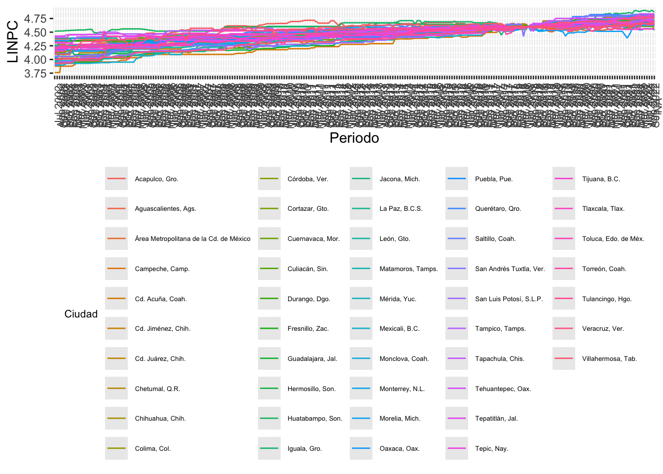
Hagamos una pruebas de Raíces Unitarias.
Change to format wide:
## # A tibble: 6 × 48
## Fecha `Acapulco, Gro.` `Aguascalientes, Ags.` Área Metropolitana de la Cd…¹
## <chr> <dbl> <dbl> <dbl>
## 1 Abr 2003 4.39 4.35 4.26
## 2 Abr 2004 4.39 4.36 4.31
## 3 Abr 2005 4.44 4.36 4.36
## 4 Abr 2006 4.47 4.33 4.40
## 5 Abr 2007 4.54 4.38 4.42
## 6 Abr 2008 4.60 4.41 4.44
## # ℹ abbreviated name: ¹`Área Metropolitana de la Cd. de México`
## # ℹ 44 more variables: `Campeche, Camp.` <dbl>, `Cd. Acuña, Coah.` <dbl>,
## # `Cd. Jiménez, Chih.` <dbl>, `Cd. Juárez, Chih.` <dbl>,
## # `Chetumal, Q.R.` <dbl>, `Chihuahua, Chih.` <dbl>, `Colima, Col.` <dbl>,
## # `Córdoba, Ver.` <dbl>, `Cortazar, Gto.` <dbl>, `Cuernavaca, Mor.` <dbl>,
## # `Culiacán, Sin.` <dbl>, `Durango, Dgo.` <dbl>, `Fresnillo, Zac.` <dbl>,
## # `Guadalajara, Jal.` <dbl>, `Hermosillo, Son.` <dbl>, …Time Series:
ts_LINPC <- ts( LINPC[c( 2:48 )],
               start = c(2002, 7),
               freq = 12)

ts_DLINPC <- diff(ts( LINPC[c( 2:48 )],
                     start = c(2002, 7),
                     freq = 12),
                  lag = 1,
                  differences = 1)
Unit Root Test: Test specifies the type of test to be performed among Levin et al. (2002), Im et al. (2003), Maddala and Wu (1999) and Hadri (2000)
Optimal lags: \[\begin{eqnarray*} p & = & Int(4*(T/100)^{(1/4)}) \\ & = & Int(4*(244/100)^{(1/4)}) \\ & = & Int(4.99) \\ & = & 4 \end{eqnarray*}\]
Consider Levin et al. (2002):
purtest(ts_LINPC, test = "levinlin", exo = "trend", # exo = c("none", "intercept", "trend"),
        lags = "AIC", pmax = 4)
##
## Levin-Lin-Chu Unit-Root Test (ex. var.: Individual Intercepts and
## Trend)
##
## data: ts_LINPC
## z = -56.022, p-value < 2.2e-16
## alternative hypothesis: stationarity
purtest(ts_DLINPC, test = "levinlin", exo = "trend", # exo = c("none", "intercept", "trend"),
        lags = "AIC", pmax = 4)
##
## Levin-Lin-Chu Unit-Root Test (ex. var.: Individual Intercepts and
## Trend)
##
## data: ts_DLINPC
## z = -107.84, p-value < 2.2e-16
## alternative hypothesis: stationarityConsider Choi (2001):
purtest(ts_LINPC, test = "logit", exo = "trend", # exo = c("none", "intercept", "trend"),
        lags = "AIC", pmax = 4)
##
## Choi's Logit Unit-Root Test (ex. var.: Individual Intercepts and Trend)
##
## data: ts_LINPC
## L* = -85.506, df = 239, p-value < 2.2e-16
## alternative hypothesis: stationarity
purtest(ts_DLINPC, test = "logit", exo = "trend", # exo = c("none", "intercept", "trend"),
        lags = "AIC", pmax = 4)
##
## Choi's Logit Unit-Root Test (ex. var.: Individual Intercepts and Trend)
##
## data: ts_DLINPC
## L* = -278.56, df = 239, p-value < 2.2e-16
## alternative hypothesis: stationarityConsider Hadri (2000):
purtest(ts_LINPC, test = "hadri", exo = "trend", # exo = c("none", "intercept", "trend"),
        lags = "AIC", pmax = 4)
##
## Hadri Test (ex. var.: Individual Intercepts and Trend) (Heterosked.
## Consistent)
##
## data: ts_LINPC
## z = -2.7, p-value = 0.9965
## alternative hypothesis: at least one series has a unit root
purtest(ts_DLINPC, test = "hadri", exo = "trend", # exo = c("none", "intercept", "trend"),
        lags = "AIC", pmax = 4)
##
## Hadri Test (ex. var.: Individual Intercepts and Trend) (Heterosked.
## Consistent)
##
## data: ts_DLINPC
## z = -8.9351, p-value = 1
## alternative hypothesis: at least one series has a unit rootEstimación PANEL con TREND:
# Modelo Final
fixed <- plm( LINPC ~ Dummy_FIRMA + Marca_01 + Marca_02 + Marca_03 + Marca_04 + Marca_05 +
              Marca_06 + Marca_07 + Marca_08 + Marca_09 + Marca_10 + Marca_11 + as.numeric(Periodo),
             data = Data,
             index=c("Ciudad", "Periodo"),
             model = "within")
## Warning in pdata.frame(data, index): at least one NA in at least one index dimension in resulting pdata.frame
## to find out which, use, e.g., table(index(your_pdataframe), useNA = "ifany")
summary(fixed)## Oneway (individual) effect Within Model
##
## Call:
## plm(formula = LINPC ~ Dummy_FIRMA + Marca_01 + Marca_02 + Marca_03 +
## Marca_04 + Marca_05 + Marca_06 + Marca_07 + Marca_08 + Marca_09 +
## Marca_10 + Marca_11 + as.numeric(Periodo), data = Data, model = "within",
## index = c("Ciudad", "Periodo"))
##
## Balanced Panel: n = 47, T = 243, N = 11421
##
## Residuals:
## Min. 1st Qu. Median 3rd Qu. Max.
## -0.4220510 -0.0416329 0.0026154 0.0471479 0.2275376
##
## Coefficients:
## Estimate Std. Error t-value Pr(>|t|)
## Dummy_FIRMA -0.05972092 0.01892851 -3.1551 0.0016087 **
## Marca_01 0.04545555 0.02069006 2.1970 0.0280423 *
## Marca_02 0.05452288 0.02372909 2.2977 0.0215956 *
## Marca_03 -0.02925504 0.02041744 -1.4328 0.1519296
## Marca_04 -0.07440826 0.02418665 -3.0764 0.0021000 **
## Marca_05 0.02633713 0.01045219 2.5198 0.0117567 *
## Marca_06 0.12521494 0.01991655 6.2870 3.356e-10 ***
## Marca_07 -0.09242328 0.02514895 -3.6750 0.0002389 ***
## Marca_08 0.03362324 0.02086579 1.6114 0.1071193
## Marca_09 0.05630828 0.02121641 2.6540 0.0079655 **
## Marca_10 -0.04866105 0.02638856 -1.8440 0.0652062 .
## Marca_11 -0.03582620 0.03031018 -1.1820 0.2372361
## as.numeric(Periodo) 0.00220384 0.00001018 216.4961 < 2.2e-16 ***
## ---
## Signif. codes: 0 '***' 0.001 '**' 0.01 '*' 0.05 '.' 0.1 ' ' 1
##
## Total Sum of Squares: 330.79
## Residual Sum of Squares: 60.08
## R-Squared: 0.81838
## Adj. R-Squared: 0.81743
## F-statistic: 3937.79 on 13 and 11361 DF, p-value: < 2.22e-16
# Modelo Final
fixed <- plm( LINPC ~ Dummy_FIRMA + as.numeric(Periodo),
             data = Data,
             index=c("Ciudad", "Periodo"),
             model = "within")
## Warning in pdata.frame(data, index): at least one NA in at least one index dimension in resulting pdata.frame
## to find out which, use, e.g., table(index(your_pdataframe), useNA = "ifany")
summary(fixed)## Oneway (individual) effect Within Model
##
## Call:
## plm(formula = LINPC ~ Dummy_FIRMA + as.numeric(Periodo), data = Data,
## model = "within", index = c("Ciudad", "Periodo"))
##
## Balanced Panel: n = 47, T = 243, N = 11421
##
## Residuals:
## Min. 1st Qu. Median 3rd Qu. Max.
## -0.4337032 -0.0421466 0.0026796 0.0480377 0.2504866
##
## Coefficients:
## Estimate Std. Error t-value Pr(>|t|)
## Dummy_FIRMA -0.02239578 0.00417897 -5.3592 0.00000008525 ***
## as.numeric(Periodo) 0.00220318 0.00001032 213.4825 < 2.2e-16 ***
## ---
## Signif. codes: 0 '***' 0.001 '**' 0.01 '*' 0.05 '.' 0.1 ' ' 1
##
## Total Sum of Squares: 330.79
## Residual Sum of Squares: 61.94
## R-Squared: 0.81275
## Adj. R-Squared: 0.81196
## F-statistic: 24680.5 on 2 and 11372 DF, p-value: < 2.22e-1610.5 Panel VAR
En esta sección extenderemos el caso del modelo VAR(p) a uno en forma panel. En este caso asumimos que las viables exogenas son los \(p\) rezagos de las \(k\) variables endogenas. Consideremos el siguiente caso de un modelo panel VAR con efectos fijos –ciertamente es posible hacer estimaciones con efectos aleatorios, no obstante requiere de supuestos adicionales que no contemplamos en estas notas –, el cual es la forma más común de estimación: \[\begin{equation} \mathbf{Y}_{it} = \mu_i + \sum_{l = 1}^p \mathbf{A}_l \mathbf{Y}_{i t - l} + \mathbf{B} \mathbf{X}_{it} + \varepsilon_{it} (\#eq:eq_PVAR) \end{equation}\]
Donde \(\mathbf{Y}_{it}\) es un vector de variables endogenas estacionarias para la unidad de corte transversal \(i\) en el tiempo \(t\), \(\mathbf{X}_{it}\) es una matriz que contiene varaibles exógenas, y \(\varepsilon_{it}\) es un término de error que cumple con: \[\begin{eqnarray*} \mathbb{E}[\varepsilon_{it}] & = & 0 \\ Var[\varepsilon_{it}] & = & \Sigma_\varepsilon \end{eqnarray*}\]
Donde \(\Sigma_\varepsilon\) es una matriz definida positiva.
Para el porceso de estimación la ecuación @ref(eq:eq_PVAR) se modifica en su versión en diferencias para quedar como: \[\begin{equation} \Delta \mathbf{Y}_{it} = \sum_{l = 1}^p \mathbf{A}_l \Delta \mathbf{Y}_{i t - l} + \mathbf{B} \Delta \mathbf{X}_{it} + \Delta \varepsilon_{it} (\#eq:eq_Dinamic_PVAR) \end{equation}\]
La ecuación @ref(eq:eq_Dinamic_PVAR) se estima por un GMM.
10.6 Ejemplos: Panel VAR(p)
Dependencies and Setup
10.6.1 Ejemplo 1
We used the dynamic panel literature by Arellano and Bond (1991), Blundell and Bond (1998) and Roodman (2009b). This data set describes employment, wages, capital and output of 140 firms in the United Kingdom from 1976 to 1984. We estimate: Employment is explained by past values of employment (“l” lags), current and first lag of wages and output and current value of capital.
##  [1] "c1"       "ind"      "year"     "emp"      "wage"     "cap"
##  [7] "indoutpt" "n"        "w"        "k"        "ys"       "rec"
## [13] "yearm1"   "id"       "nL1"      "nL2"      "wL1"      "kL1"
## [19] "kL2"      "ysL1"     "ysL2"     "yr1976"   "yr1977"   "yr1978"
## [25] "yr1979"   "yr1980"   "yr1981"   "yr1982"   "yr1983"   "yr1984"
## c1 ind year emp wage cap indoutpt n w k
## 1 1-1 7 1977 5.041 13.1516 0.5894 95.7072 1.617604 2.576543 -0.5286502
## 2 2-1 7 1978 5.600 12.3018 0.6318 97.3569 1.722767 2.509746 -0.4591824
## 3 3-1 7 1979 5.015 12.8395 0.6771 99.6083 1.612433 2.552526 -0.3899363
## 4 4-1 7 1980 4.715 13.8039 0.6171 100.5501 1.550749 2.624951 -0.4827242
## 5 5-1 7 1981 4.093 14.2897 0.5076 99.5581 1.409278 2.659539 -0.6780615
## 6 6-1 7 1982 3.166 14.8681 0.4229 98.6151 1.152469 2.699218 -0.8606195
## ys rec yearm1 id nL1 nL2 wL1 kL1 kL2
## 1 4.561294 1 1977 1 NA NA NA NA NA
## 2 4.578383 2 1977 1 1.617604 NA 2.576543 -0.5286502 NA
## 3 4.601245 3 1978 1 1.722767 1.617604 2.509746 -0.4591824 -0.5286502
## 4 4.610656 4 1979 1 1.612433 1.722767 2.552526 -0.3899363 -0.4591824
## 5 4.600741 5 1980 1 1.550749 1.612433 2.624951 -0.4827242 -0.3899363
## 6 4.591224 6 1981 1 1.409278 1.550749 2.659539 -0.6780615 -0.4827242
## ysL1 ysL2 yr1976 yr1977 yr1978 yr1979 yr1980 yr1981 yr1982 yr1983
## 1 NA NA 0 1 0 0 0 0 0 0
## 2 4.561294 NA 0 0 1 0 0 0 0 0
## 3 4.578383 4.561294 0 0 0 1 0 0 0 0
## 4 4.601245 4.578383 0 0 0 0 1 0 0 0
## 5 4.610656 4.601245 0 0 0 0 0 1 0 0
## 6 4.600741 4.610656 0 0 0 0 0 0 1 0
## yr1984
## 1 0
## 2 0
## 3 0
## 4 0
## 5 0
## 6 0Estimación
#?pvargmm

Arellano_Bond_1991_table4b <- pvargmm( dependent_vars = c("n"),
                                       lags = 2,
                                       exog_vars = c("w", "wL1", "k", "ys", "ysL1", "yr1979", "yr1980", "yr1981", "yr1982",
                                                      "yr1983", "yr1984"),
                                       transformation = "fd", data = abdata,  panel_identifier = c("id", "year"),
                                       steps = c("twostep"),
                                       system_instruments = FALSE,
                                       max_instr_dependent_vars = 99,
                                       min_instr_dependent_vars = 2L,
                                       collapse = FALSE)
summary(Arellano_Bond_1991_table4b)Dynamic Panel VAR estimation, two-step GMM
Transformation: First-differences
Group variable: id
Time variable: year
Number of observations = 611
Number of groups = 140
Obs per group: min = 4
Obs per group: avg = 4.36428571428571
Obs per group: max = 6
Number of instruments = 38
| n | |
|---|---|
| lag1_n | 0.4742* |
| (0.1854) | |
| lag2_n | -0.0530 |
| (0.0517) | |
| w | -0.5132*** |
| (0.1456) | |
| wL1 | 0.2246 |
| (0.1419) | |
| k | 0.2927*** |
| (0.0626) | |
| ys | 0.6098*** |
| (0.1563) | |
| ysL1 | -0.4464* |
| (0.2173) | |
| yr1979 | 0.0105 |
| (0.0099) | |
| yr1980 | 0.0247 |
| (0.0158) | |
| yr1981 | -0.0158 |
| (0.0267) | |
| yr1982 | -0.0374 |
| (0.0300) | |
| yr1983 | -0.0393 |
| (0.0347) | |
| yr1984 | -0.0495 |
| (0.0349) | |
| ***p < 0.001; **p < 0.01; *p < 0.05 | |
Instruments for equation
Standard
w, wL1, k, ys, ysL1, yr1979, yr1980, yr1981, yr1982, yr1983, yr1984
GMM-type
Dependent vars: L(2,6))
Collapse = FALSE
Hansen test of overid. restrictions: chi2(25) = 30.11 Prob > chi2 = 0.22
(Robust, but weakened by many instruments.)
10.6.2 Ejemplo 2:
We used the panel data set consists of 265 Swedish municipalities and covers 9 years (1979-1987). These variables include total expenditures (expenditures), total own-source revenues (revenues) and intergovernmental grants received by the municipality (grants). Source: Dahlberg and Johansson (2000)
Grants from the central to the local government are of three kinds: support to municipalities with small tax capacity, grants toward the running of certain local government activities and grants toward certain investments.
## [1] "id" "year" "expenditures" "revenues" "grants"
head(Dahlberg)## id year expenditures revenues grants
## 1 114 1979 0.0229736 0.0181770 0.0054429
## 2 114 1980 0.0266307 0.0209142 0.0057304
## 3 114 1981 0.0273253 0.0210836 0.0056647
## 4 114 1982 0.0288704 0.0234310 0.0058859
## 5 114 1983 0.0226474 0.0179979 0.0055908
## 6 114 1984 0.0215601 0.0179949 0.0047536Estimación:
ex1_dahlberg_data <- pvargmm(dependent_vars = c("expenditures", "revenues", "grants"),
          lags = 1,
          transformation = "fod",
          data = Dahlberg,
          panel_identifier=c("id", "year"),
          steps = c("twostep"),
          system_instruments = FALSE,
          max_instr_dependent_vars = 99,
          max_instr_predet_vars = 99,
          min_instr_dependent_vars = 2L,
          min_instr_predet_vars = 1L,
          collapse = FALSE
  )
## Warning in pvargmm(dependent_vars = c("expenditures", "revenues", "grants"), :
## The matrix D_e is singular, therefore the general inverse is used
summary(ex1_dahlberg_data)Dynamic Panel VAR estimation, two-step GMM
Transformation: Forward orthogonal deviations
Group variable: id
Time variable: year
Number of observations = 1855
Number of groups = 265
Obs per group: min = 7
Obs per group: avg = 7
Obs per group: max = 7
Number of instruments = 252
| expenditures | revenues | grants | |
|---|---|---|---|
| lag1_expenditures | 0.2846*** | 0.2583** | 0.0167 |
| (0.0664) | (0.0795) | (0.0172) | |
| lag1_revenues | -0.0470 | 0.0588 | -0.0405** |
| (0.0637) | (0.0726) | (0.0151) | |
| lag1_grants | -1.6746*** | -2.2367*** | 0.3204*** |
| (0.2818) | (0.2846) | (0.0521) | |
| ***p < 0.001; **p < 0.01; *p < 0.05 | |||
Instruments for equation
Standard
GMM-type
Dependent vars: L(2,7))
Collapse = FALSE
Hansen test of overid. restrictions: chi2(243) = 263.01 Prob > chi2 = 0.18
(Robust, but weakened by many instruments.)
Model selection procedure of Andrews and Lu (2001) to select the optimal lag length for our example
Andrews_Lu_MMSC(ex1_dahlberg_data)## $MMSC_BIC
## [1] -1610.877
##
## $MMSC_AIC
## [1] -234.9924
##
## $MMSC_HQIC
## [1] -792.3698
ex2_dahlberg_data <- pvargmm(dependent_vars = c("expenditures", "revenues", "grants"),
                             lags = 2,
                             transformation = "fod",
                             data = Dahlberg,
                             panel_identifier=c("id", "year"),
                             steps = c("twostep"),
                             system_instruments = FALSE,
                             max_instr_dependent_vars = 99,
                             max_instr_predet_vars = 99,
                             min_instr_dependent_vars = 2L,
                             min_instr_predet_vars = 1L,
                             collapse = FALSE)
## Warning in pvargmm(dependent_vars = c("expenditures", "revenues", "grants"), :
## The matrix D_e is singular, therefore the general inverse is used
summary(ex2_dahlberg_data)Dynamic Panel VAR estimation, two-step GMM
Transformation: Forward orthogonal deviations
Group variable: id
Time variable: year
Number of observations = 1590
Number of groups = 265
Obs per group: min = 6
Obs per group: avg = 6
Obs per group: max = 6
Number of instruments = 243
| expenditures | revenues | grants | |
|---|---|---|---|
| lag1_expenditures | 0.2572** | 0.2486* | 0.0135 |
| (0.0893) | (0.1018) | (0.0178) | |
| lag1_revenues | -0.1219 | -0.0634 | -0.0293 |
| (0.0879) | (0.0997) | (0.0171) | |
| lag1_grants | -3.0718*** | -3.5849*** | 0.1581* |
| (0.5941) | (0.6168) | (0.0636) | |
| lag2_expenditures | -0.0247 | 0.0252 | 0.0178 |
| (0.0791) | (0.0834) | (0.0157) | |
| lag2_revenues | -0.2584** | -0.2446** | -0.0237 |
| (0.0785) | (0.0800) | (0.0157) | |
| lag2_grants | -1.5265*** | -1.6687*** | 0.0702 |
| (0.1873) | (0.2113) | (0.0586) | |
| ***p < 0.001; **p < 0.01; *p < 0.05 | |||
Instruments for equation
Standard
GMM-type
Dependent vars: L(2,6))
Collapse = FALSE
Hansen test of overid. restrictions: chi2(225) = 260.11 Prob > chi2 = 0.054
(Robust, but weakened by many instruments.)
Andrews_Lu_MMSC(ex2_dahlberg_data)## $MMSC_BIC
## [1] -1486.935
##
## $MMSC_AIC
## [1] -213.8917
##
## $MMSC_HQIC
## [1] -734.1071Sstability of the autoregressive process:
## Eigenvalue stability condition:
##
##              Eigenvalue    Modulus
## 1 0.5370657+0.00000000i 0.53706574
## 2 0.0633651+0.06442426i 0.09036383
## 3 0.0633651-0.06442426i 0.09036383
##
## All the eigenvalues lie inside the unit circle.
## PVAR satisfies stability condition.
plot(stab_ex1_dahlberg_data)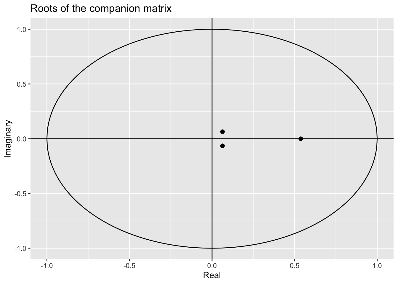
Generate impulse response functions.
# ex1_dahlberg_data_oirf <-  oirf(ex1_dahlberg_data, n.ahead = 8)
#
# ex1_dahlberg_data_girf <-  girf(ex1_dahlberg_data, n.ahead = 8, ma_approx_steps= 8)
#
# ex1_dahlberg_data_bs <-  bootstrap_irf(ex1_dahlberg_data, typeof_irf = c("GIRF"),
#                                        n.ahead = 8,
#                                        nof_Nstar_draws = 500,
#                                        confidence.band = 0.95)
#
# plot(ex1_dahlberg_data_girf, ex1_dahlberg_data_bs)